So let’s describe the game we’re playing here and give it some notation.
We have some agent \(\pi\) - say a robot or a human being or whatever. Something or someone that is clever and can make decisions.
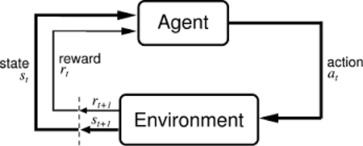
This agent makes decisions or performs actions based on some set of observations \(o\) that depend on some state \(s\) of the environment. The environment is the world in which the agent lives.
For the sake of simplicity assume the agent can observe everything about the state of the environment
For example in the case of a self driving car: the agent is the car’s brain. The car observes an image of the road of infront of it; this image describes the state of the environment. Based on this image- it makes a decision of turning left, right or going straight.
The environment/world takes this action and current state and produces a new state - which is the new image the car sees after it has moved in some direction. And this game goes on for T time steps.
The environment may also throw out some sort of reward. The reward can be thought of the outcome of the action. In this example the reward can be binary. Crashed or not crashed.
Pictorally:
We begin with state \(s_0\) and reward \(r_0\). The car observe this picture and reward; and goes a cetrain direction \(a_0\), based on policy \(\pi\) which leads to a new image \(s_1\) and a new reward \(r_1\).
Our goal is to be able to learn a general policy to maximize our reward. Simply put we’d like to learn a policy which the car can use to not crash while driving.
Before we formalize what learning a policy we mean- what does a policy look like? The answer is that it depends - the most generalized assumption is that all policies are drawn from some unknow policy distribution \(\pi\) and this distribution is parameterized by some set of weights \(\theta\).
The agents actionas are drawn from the conditional distribution of said policy i.e
\(\pi_{\theta}(a_t | s_t)\) can be thought of the probability of playing action \(a_t\) when seeing state \(s_t\)
Learning an optimal policy refers to learning some optimal set of weights \(\theta^*\) such that when we choose actions based on this policy we obtain the most cumulative reward we could’ve obtained.
Notation:
Our goal is to find a policy that maximises expected reward which is to say:
\[\begin{align*} \theta^* &= \text{argmax}_{\theta} \mathbb{E}_{(\tau) \sim p(\tau)} \Big( \sum_{t=1}^T r(s_t, a_t) \Big) \\ \ &= \text{argmax}_{\theta} \mathbb{E}_{(a_1, s_1, ..., a_T, s_T) \sim p(a_1, s_1, ..., a_T, s_T)} \Big( \sum_{t=1}^T r(s_t, a_t) \Big) \end{align*}\]Note since everything is random, we look to maximize the expected cumulatitve reward over the joint distribution of all actions.
The above equation can be re-written as
\[\begin{align*} \theta^* &= \text{argmax}_{\theta} \sum_{t} \text{ } \mathbb{E}_{(a_t, s_t) \sim p(a_t, s_t)} [ \text{ } r(s_t, a_t) ] \end{align*}\]where \((a_t, s_t)\) is the marginal probability distribution over the joint.
To see why visit
We define Q function of a policy as:
\[\begin{align*} Q^{\pi}(s_t, a_t) &= r(s_t, a_t) + \sum_{i=t+1}^{T} \mathbb{E}_{a_i \sim \pi(a_i | s_i)}\Big(r(s_i, a_i) | s_t, a_t\Big) \end{align*}\]If I take action \(a_t\) when in state \(s_t\) and from then use policy \(\pi\): what is the cumulative cumulative reward I get in expectation. As the policy is random- we don’t know for sure what reward we’d get in the future states.
We define Value function as the Expectation over Q.
\[\begin{align*} V^{\pi}(s_t) &= \sum_{i=t}^{T} \mathbb{E}_{a_i \sim \pi(a_i | s_i)}[r(s_i, a_i) | s_t] \\ &= \mathbb{E}_{a_t \sim \pi(a_t | s_t)} Q(s_t, a_t) \end{align*}\]If we start in state t; then use the policy what is the reward we get.
Note the only difference between Q and V is that at state t; Q specifies an action whereas V does not. So the the cumulative regret is averaged over all possible actions at state t in V whereas it isn’t for Q. This maves V just the expected value of Q
It is the Easy to show that the the final optimization problem is just the value of the policy starting at state 1
\[\theta^* = \text{argmax}_{\theta} \text{ } \mathbb{E}_{s_1 \sim p(s_1)} \text{ }V(s_1) \]
Note we can bring K in as it is just constant relative to the variables with which we’re taking expectations.
\[\begin{align*} \theta^* = \text{argmax}_{\theta} \text{ } \mathbb{E}_{s_1 \sim p(s_1)} \text{ }V(s_1) \end{align*}\]