These are my notes for Efficient Neural Architechture search - ENAS
Just a high level overview of the main idea. Will not go into details of each
In an earlier writeup I described the setting of learning hyperparameters using the Reinforce algorithm.
Quick recap: start with some random configurations of convolutional neural networks. You train them till convergence and evaluate their performance on some validation set. These configurations can be described as a sequence of tokens. Feed these sequences and the validation accuracies to an RNN controller to produce new sequences. Use these sequences as the new configuration and repeat.
One of the downsides of this approach as mentioned in the paper is it takes 450 GPU’s and 3 days to train the model end to end. So unless you’re Mother Google or one of the other big tech companies - good luck coding this up.
In this paper they authors show us how to get the same results using 1 1080 TI GPU and 7 hours of training.
Well close to everything. So it’s probably more productive not relating this part to the earlier post and pretend this is it’s separate idea.
“Central to the idea of ENAS is the observation that all of the graphs which NAS ends up iterating over can be viewed as sub-graphs of a larger graph”
So say we define some graph where each node defines some compuation.
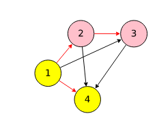
Take for example, in the picture below, node 1 represents 5x5 convolution with certain stride and padding. Node 2 represents an activation function like RELU or sigmoid and so on. One can construct a neural network by subsampling nodes in this big graph and sticking them together.
The red lines depict the edges the controller have sampled from the big DAG to propse an architechture.
This pretty much what efficient NAS is. Now the search space is restricted by the big DAG instead of the vocabulary of sequences in the original NAS paper. While the search space than NAS it is not trivially small. NAS produces networks with roughly 54 million parameters as opposed to 24 million parameters produced by ENAS.
So where is the gain coming from? The next section illustrates the key idea.
Going back to picture above.
Each node in the big DAG defines a computation. Say node 1 is the input, node 2 is a convolution, node 3 and node 4 is yet another convolution. As node 1 is the input there is nothing to do there. In node 2, say we can have a 3x3 convolution or 5x5 convolution. Node 3 defines some activation - either relu or sigmoid. There are a total of 4 possible dataflow paths between node 2 and node 3. Namely:
The job of the controller is to sample one of these paths. In the paper they say, we note that for each pair of nodes \(j < ℓ\) , there is an independent parameter matrix \(W^h_{ℓ,j}\). By choosing the previous indices, the controller also decides which parameter matrices are used. Therefore, in ENAS, all recurrent cells in a search space share the same set of parameters.
So unlike in the original NAS where each recurrent cell could recommend an indepent kernel/weight matrix to learn; here there is a finite number of weights to learn and they’re all shared by the recurrent cells. This is somewhat confusing to me?
What happens when you learn a certain subgraph and sample another subgraph that uses the previous subgraph partially? Do you relearn the weights or use the old ones? Refer to confusion section.
The controller looks pretty much the same as NAS. It’s a seq-to-seq model using some RNN (LSTM or GRU or whatver). Each node in the big graph corresponds to a RNN cell in the controller. At each cell the controller does two things- sample previous nodes it should connect to (this leads to skip connections) and decides which computation defined by that node to sample.
There is hyper optimization technique called hyperband which essentially goes through random configurations and drops the poor performing configurations at regular intervals. Eventually the goal is to converge to the right configuration. Can you use the DAG as a prior to sample from and eliminate the controller? So instead of reinforcement learning build a clever prior and then sample randomly.
There’s still a lot of parameters to learn. It’s unclear to me where the speedup is coming from. Do they start from the previously learned weight every time? Or they stop learning and just stitch together nodes after some time?
Here’s what they say:
The main contribution of this work is to improve the efficiency of NAS by forcing all child models to share weights to eschew training each child model from scratch to convergence. The idea has apparent complications, as different child models might utilize their weights differently, but was encouraged by previous work on transfer learning and multitask learning, which established that parameters learned for a particular model on a particular task can be used for other models on other tasks, with little to no modifications ( Razavian et al. , 2014 ; Zoph et al. , 2016 ; Luong et al. , 2016 ).
If they are just learning the parameters once - which would give them a tonne of speedup then this is pretty much saying each convolution layer is close to independent of anything but the previous layer. So is this like a markov assumption.
Is this secretly another Baysian hyperoptimization paper? I have to think about this one.