These are my notes, and implementation of Neural Architechture search
Most of the times in machine learning you want to train model to be able to perform some task. For example, you may want to train a convolutional neural network to be able to predict if a given image is a picture Lionel Messi or not.
If you could accurately learn the weights(parameters) of said neural network you’d be able to predict with reasonable accuracy if an image is that of Leo Messi or not.
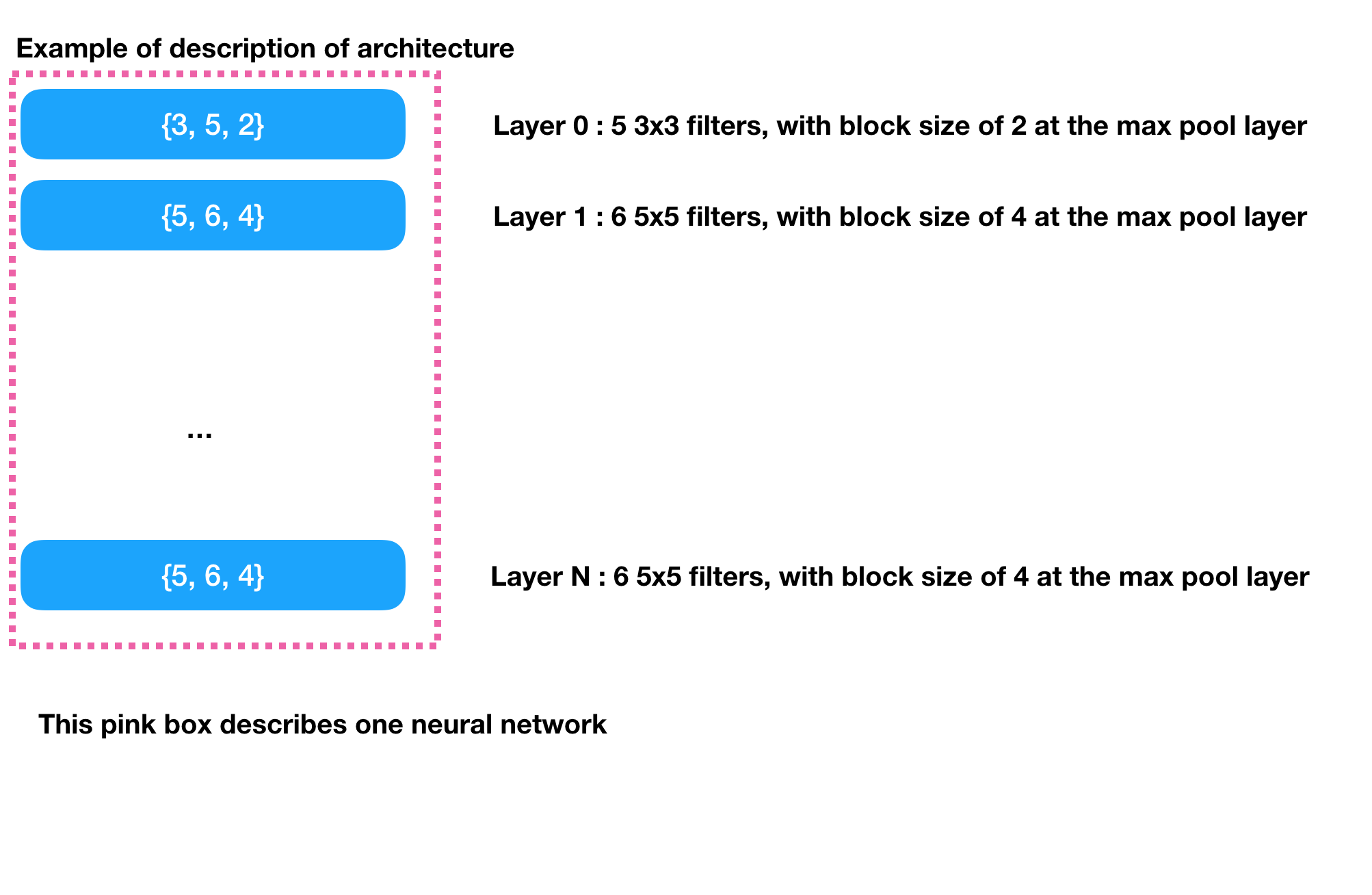
However before you even learn the weights of neural network you need to decide on the structure of it. The structure is given by what we call hyper parameters. For a convolutional neural network hyperparameters can be of the form:
For a more detailed introduction to convolutional neural networks visit
The parameters of a neural network are usually learned by solving some sort of optimization problem by stochastic gradient descent.
In the classical setting the hyperparameters are learned by guessing i.e a human expert decides the structure; we learn the weights and look at validation accuracy on a test set. Then we try a different architechture and repeat the process.
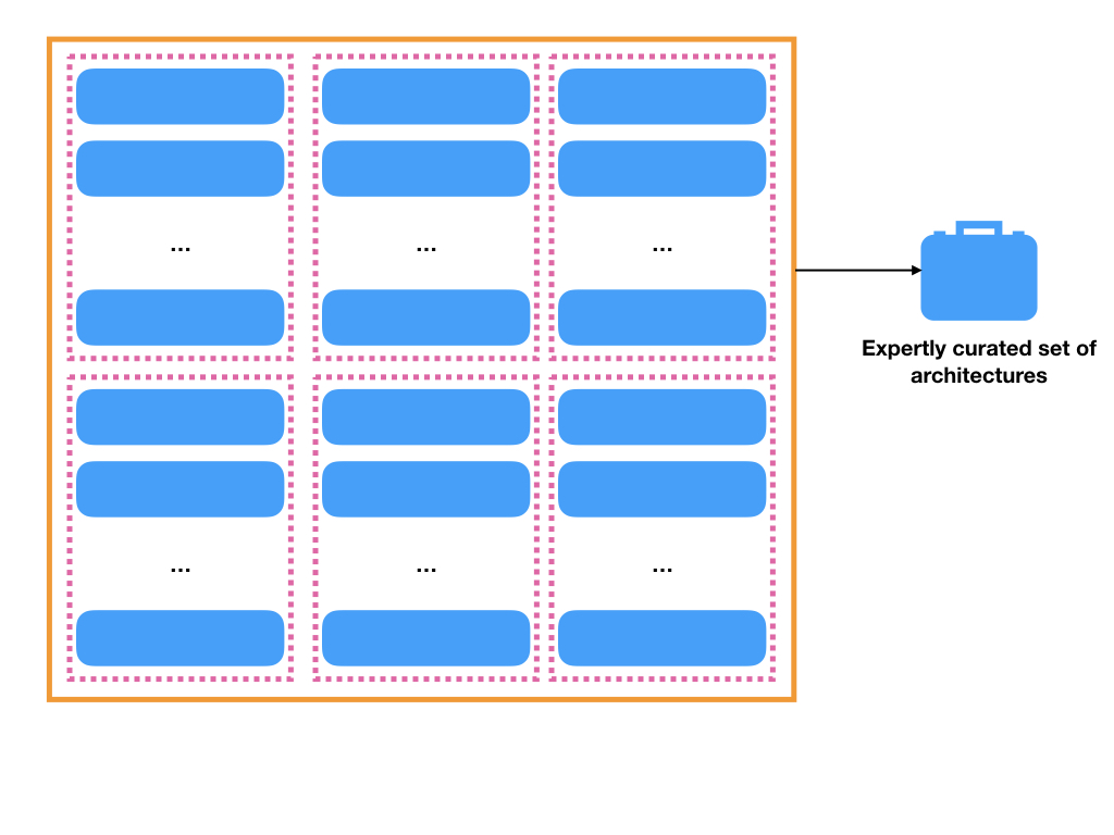
I view it as a search through a finite set of possible architechtures. The set is crafted by experts using intuition and experience.
Crafting this finite set turns out be very time consuming and a giant pain in the backside. So the people at Google recommend we let another learning algorithm solve this problem for us. So instead of trying architechtures carefully crafted by experts - try architechtures recommended by another learning algorithm. This is the whole idea behind Neural Architechture search- NAS
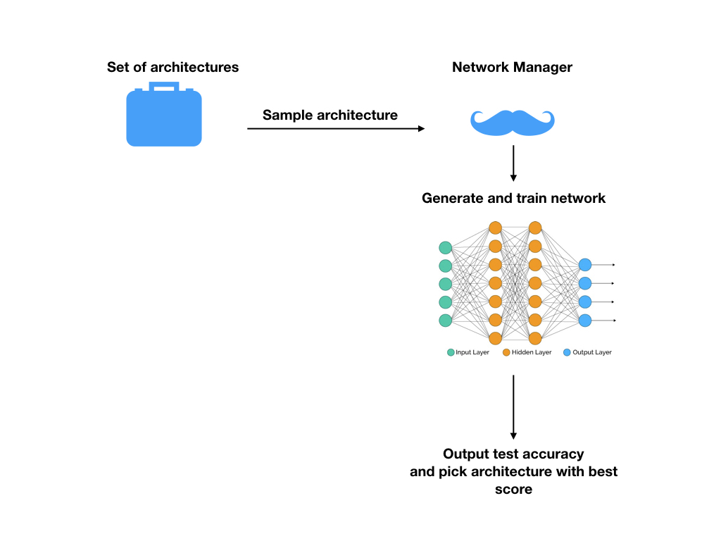
Here’s what the training picture looks like:
An example of what hyperparameters look like
An expert picks a set of different networks
He uses the architechture with the best test accuracy
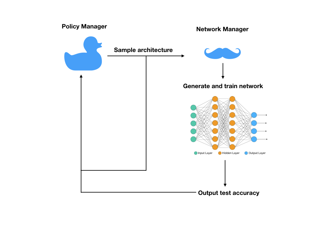
Now we introduce a policy manager with searches through an infinite set of architechtures and makes recommendations based on how well we’ve been doing so far.
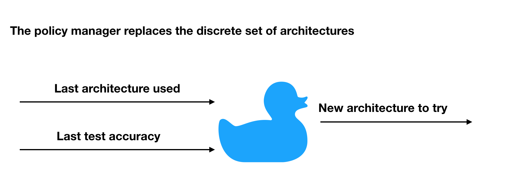
The full picture
Training the policy manager is the new gig in this paper. This is done by an algorithm known as policy gradient descent. Before I delve into the details it’s useful to understand it in relation to the classical supervised learning setting we’re more used to.
If I were to learn a policy using immitation learning this is how I’d go about it:
Statistically we’re just doing maximum likelihood estimation:
We have some likelihood distribution \(\pi_{\theta}(a_t|s_t)\) and we want the find the parameters \(\hat{\theta}\) that maximize this likelihood
Make a note of this equation as it’ll be useful to understand why we go through all the steps for policy gradient.
Learning the parameters of the policy network can be viewed as an instance of reinforcement learning. At each time step we produce an actions i.e the architechtures to use - those architechtures have validation accuracies which can be treated as rewards and fed back into the policy network. In this case the state space and the action space of the reinforcing agent is the same - description of the neural network.
Sticking to notation I used in my notes for RL learning we have
\(s_t\) as the architechtures used in time step t and \(r_t\) as the rewards for those architechtures.
\(a_t\) = \(s_{t+1}\) is the architechture generated by our policy network \(\pi\) which is parameterized by \(\theta\).
I.e the goal is to learn values for \(\theta\) so our rewards are maximized which from the previous set of notes boils down to :
\[\begin{align*} \theta^* &= \text{argmax}_{\theta} \mathbb{E}_{\tau \sim \pi_{\theta}(\tau)} \Big( \sum_{t=1}^T r(s_t, a_t) \Big) \\ \text{Clearing up some notation}\\ &= \text{argmax}_{\theta} \mathbb{E}_{\tau \sim \pi_{\theta}(\tau)} \Big( r(\tau) \Big) \\ &= \text{argmax}_{\theta} J(\theta) \\ \end{align*}\]So we have:
\[\begin{align*} J(\theta) &= \mathbb{E}_{\tau \sim \pi_{\theta}(\tau)} \Big( r(\tau) \Big)\\ &= \int \pi_{\theta}(\tau) r(\tau) d\tau \\ \nabla J(\theta)&= \int \nabla\pi_{\theta}(\tau)r(\tau) d\tau \\ &= \int \Big(\pi_{\theta}(\tau) \nabla log\pi_{\theta}(\tau) \Big) r(\tau) d\tau \\ \text{Since by chain rule} \\ \pi_{\theta}(\tau)\nabla log\pi_{\theta}(\tau) &= \pi_{\theta}(\tau)\frac{\nabla\pi_{\theta}(\tau)}{\pi_{\theta}(\tau)} \\ &= \nabla\pi_{\theta}(\tau) \end{align*}\]Therefore we finally have
\[\begin{align*} \nabla J(\theta) &= \int \Big( \pi_{\theta}(\tau)\nabla log\pi_{\theta}(\tau) \Big) r(\tau) d\tau \\ &= \mathbb{E}_{\tau \sim \pi_{\theta}(\tau)}\Big( \nabla log\pi_{\theta}(\tau) r(\tau) \Big) \end{align*}\]Due to the dependency graph of MDP’s it is easy to show (derivation jut a simple application of Bayes theorem and conditional independence):
\[\begin{align*} \pi_{\theta}(a_1, s_1, ..., a_T,s_T) &= p(s_1)\prod_{i=1}^T \pi_{\theta}(a_i | s_i)p(s_{i+1} | s_i, a_i) \end{align*}\]where p is the unknown reward distribution of the environment in general and in this case is the likelihood of the learned neural network.
\[\begin{align*} \pi_{\theta}(a_1, s_1, ..., a_T,s_T) &= p(s_1)\prod_{i=1}^T \pi_{\theta}(a_i | s_i)p(s_{i+1} | s_i, a_i) \\ \text{Taking log on both sides} \\ log \pi_{\theta}(\tau) &= \log p(s_1) + \sum_{i=1}^T log\pi_{\theta}(a_i | s_i) + logp(s_{i+1} | s_i, a_i) \\ \text{Taking gradient w.r.t } \theta \\ \nabla log \pi_{\theta}(\tau) & = \sum_{i=1}^T \nabla log\pi_{\theta}(a_i | s_i) \end{align*}\]So finally the gradient of our objective function looks like:
\[\begin{align*} \nabla J(\theta) &= \mathbb{E}_{\tau \sim \pi_{\theta}(\tau)}\Big( \nabla log\pi_{\theta}(\tau) r(\tau) \Big)\\ & = \mathbb{E}_{\tau \sim \pi_{\theta}(\tau)}\Big( \sum_{i=1}^T \nabla log\pi_{\theta}(a_i | s_i)r(\tau) \Big) \\ \text{Substituting in $r(\tau)$ from earlier} \\ & = \mathbb{E}_{\tau \sim \pi_{\theta}(\tau)}\Big( \sum_{i=1}^T \nabla log\pi_{\theta}(a_i | s_i)\sum_{t=1}^T r(s_t, a_t) \Big) \\ \end{align*}\]It’s important to note we’ve eliminated all dependence on the environment distribution p. It could be as ugly as possible and it doesn’t matter for gradient calcuation.
Now we still don’t know the joint distrubution \(\tau\) so we can’t compute the expectation analytically but we seldom do in modern machine learning. Solution just do monte carlo
\[\begin{align*} \nabla J(\theta) &\simeq \frac{1}{N}\sum_{k=1}^N\Big( \sum_{i=1}^T \nabla log\pi_{\theta}(a_{k,i} | s_{k,i})\sum_{t=1}^T r(s_{k,t}, a_{k,t}) \Big) \end{align*}\]The above quantity is easily computable and we can perform gradient ascent:
\[ \theta_{i+1} = \theta_i + \alpha \nabla J(\theta)\]
Why did i go through the pain of typing so much algebra ? The reason for doing derivation is to understand the relationship of policy gradient with the classical maximum likelihood estimation which we’re used to in supervised learning.
Go back to the immitation learning situation where the only difference is we don’t account for the rewards in between.
The picture looks like this:
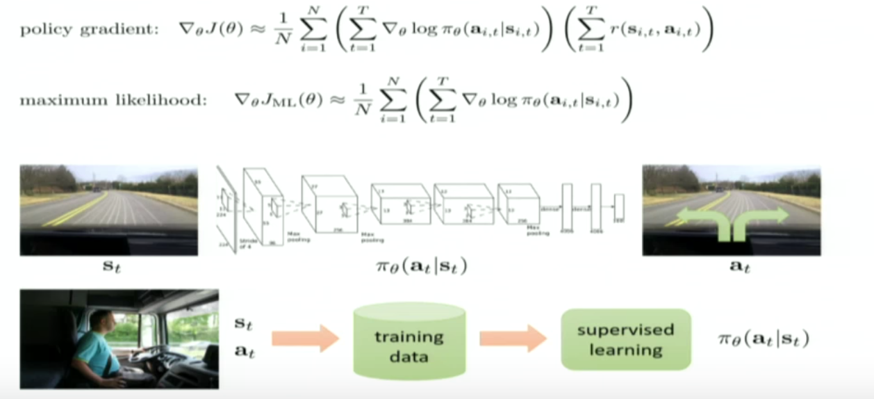
(Stolen from the Berkely course for deep reinforcement learning: only cos I didn’t want to type out that much Tex anymore)
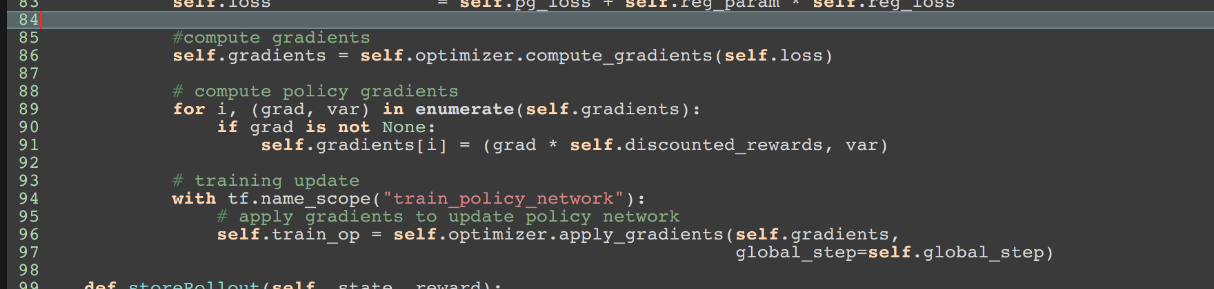
Notice the policy gradient is the exact same thing as the likelihood gradient just weighted by the rewards. So if we have a framework like tensorflow which gives us the likelihood gradients - we can just weight them by the rewards to get the policy gradient update.
So hardly any infrastructure change is required. A snapshot of such a transformation is provided below.
A simple fully functioning version of NAS is availbale here. It was written with a lot of guidance from this blog
I’d like to reference this very well written post which details why I’m skeptical this will work. It articulates some of the biggest concerns with example. One of the big points worht mentioning is: “Are those extremely long CPU hours worth the gain when we aren’t sure if we’ve even generalized?”
Recurrent networks are really hard to train. So to assume we can train a policy manager and several non convex learned models at each timestep seems hard to believe.
However haveing said everything above mother google says all this is a good idea- mother google has also published papers saying they have better test accuracy on datasets - mother google is often right so it is what it is and I timidly get on the bandwagon.
Policy gradient in it’s vanilla form (reinforce) doesn’t really work. It needs variance reduction techqniques
TODO
The paper trains multiple architechtures at one time steps. My code is linear. It needs to be made distributed